作者：昇腾实战派
知识地图：Ascend（昇腾）性能优化文章导航

背景概述

2026年，千问发布了Qwen3.5系列模型，其中MoE模型参数量更大，语义理解能力更强，同时由于每次前向计算只激活少量专家，推理速度有所保障。

本文将围绕Qwen3.5模型的MoE部分展开，内容包括参数分析、结构分析、vllm实现流程和profiling拆解方法。

本文基于transforms仓和vllm、vllm-ascend框架代码分析，请以官方代码仓为准。

一、模型参数

Qwen3.5系列中，397B/122B/35B为MoE模型，它们的模型结构相似，主要区别体现在各参数上。Qwen3.5 MoE模型的主要参数如表1所示，其区别体现在模型层数、隐藏层维度、MoE专家数、激活专家数和专家中间维度上。

参数项	Qwen3.5-397B-A17B	Qwen3.5-122B-A10B	Qwen3.5-35B-A3B
总参数量	397B	122B	35B
每步激活参数	17B	10B	3B
激活比例	~4.3%	~8.2%	~8.6%
网络层数	60	48	40
隐藏维度	4096	3584	2816
词表大小	248320	248320	248320
MoE 总专家数	512	256	256
激活专家数	11（10 路由 + 1 共享）	9（8 路由 + 1 共享）	9（8 路由 + 1 共享）
专家中间维度	1024	1024	512
原生上下文	262144（256K）	262144（256K）	262144（256K）

表1 Qwen3.5 MoE模型参数比较

二、模型结构

Qwen3.5-397B模型结构如图1所示。该模型包含60个DecodeLayer，其中每个DecodeLayer由两个ResNet组成，第一个ResNet做RMSNorm+attention，第二个ResNet做RMSNorm+MoE。可以把模型结构分为以下关键部分：

**（1）混合Attention：**Qwen3.5模型的Attention计算分为两类，分别是Gated DeltaNet和Gated Attention，两者的占比为3:1。其中，Gated Attention与Qwen3系列模型Attention基本一致，为GQA结构。

**（2）MoE：**将模型FFN 前馈层拆分为大量独立“专家子网络”，通过路由为不同语义的 Token​按需激活少量专家​，实现​稀疏计算​。

**（3）MTP：**借助草稿模型实现一次前向传播，同时预测未来多个 token，从而加快推理速度。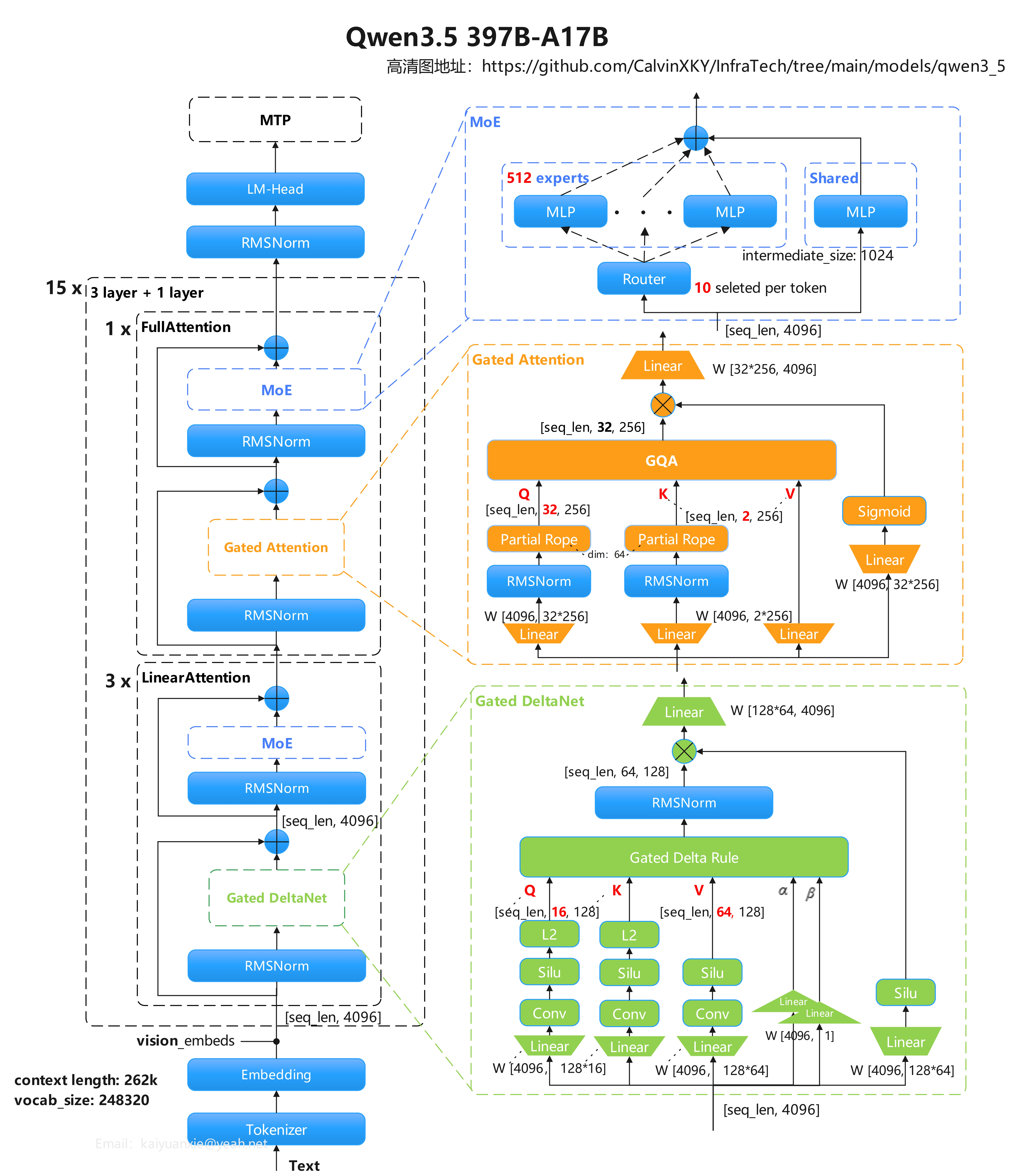

图1 Qwen3.5-397B 模型结构

与dense模型相比，MoE模型唯一的区别在于使用MoE层代替了各DecodeLayer中的FFN层。MoE层通过引入多个专家，提升模型容量和表达能力，可以学习到更加细粒度的知识；通过门控网络稀疏激活，在大幅增加参数量的同时控制计算成本，提升推理效率。

三、MoE结构

3.1 概述

transformers仓中的Qwen3_5MoeSpareMoeBlock是MoE层的实现类。其源码如下：

class Qwen3_5MoeSparseMoeBlock(nn.Module):
    def __init__(self, config):
        super().__init__()
        self.gate = Qwen3_5MoeTopKRouter(config)
        self.experts = Qwen3_5MoeExperts(config)
        self.shared_expert = Qwen3_5MoeMLP(config, intermediate_size=config.shared_expert_intermediate_size)
        self.shared_expert_gate = torch.nn.Linear(config.hidden_size, 1, bias=False)

    def forward(self, hidden_states: torch.Tensor) -> tuple[torch.Tensor, torch.Tensor]:
        batch_size, sequence_length, hidden_dim = hidden_states.shape
        hidden_states_reshaped = hidden_states.view(-1, hidden_dim)
        shared_expert_output = self.shared_expert(hidden_states_reshaped)
        _, routing_weights, selected_experts = self.gate(hidden_states_reshaped)
        expert_output = self.experts(hidden_states_reshaped, selected_experts, routing_weights)

        shared_expert_output = F.sigmoid(self.shared_expert_gate(hidden_states_reshaped)) * shared_expert_output

        expert_output = expert_output + shared_expert_output
        expert_output = expert_output.reshape(batch_size, sequence_length, hidden_dim)
        return expert_output

计算流程如图2所示。输入经过重排后，一方面经过共享专家处理并激活，得到门控共享专家输出，另一方面先经过门控/路由模块选择待激活的路由专家，再把输入交给选中的路由专家计算，得到路由专家输出。将共享专家输出和路由专家输出相加再重排，得到最终结果。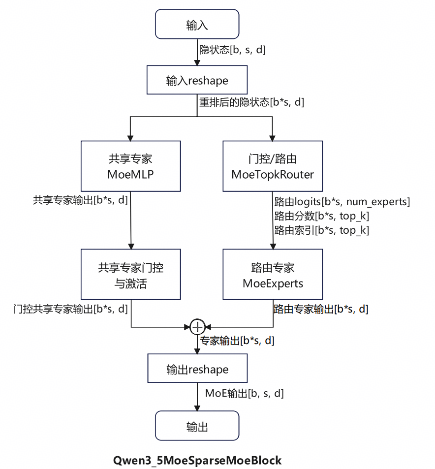

图2 Qwen3_5MoeSpareMoeBlock 流程图

3.2 共享专家实现

共享专家实现类为Qwen3_5MoeMLP。

class Qwen3_5MoeMLP(nn.Module):
    def __init__(self, config: Qwen3_5MoeConfig, intermediate_size: int):
        super().__init__()
        self.config = config
        self.hidden_size = config.hidden_size
        self.intermediate_size = intermediate_size
        self.gate_proj = nn.Linear(self.hidden_size, self.intermediate_size, bias=False)
        self.up_proj = nn.Linear(self.hidden_size, self.intermediate_size, bias=False)
        self.down_proj = nn.Linear(self.intermediate_size, self.hidden_size, bias=False)
        self.act_fn = ACT2FN[config.hidden_act]

    def forward(self, x):
        down_proj = self.down_proj(self.act_fn(self.gate_proj(x)) * self.up_proj(x))
        return down_proj

其中，由于config.json文件指定"hidden_act": “silu”，此处的ACT2FN为silu。

计算流程如图3所示。重排后的输入经门控投影和silu激活后，与上投影结果按元素相乘，再做下投影，得到共享专家输出。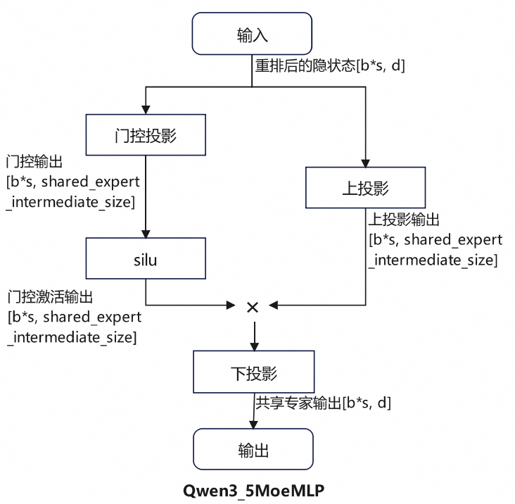

图3 Qwen3_5MoeMLP 流程图

3.3 共享专家门控与激活

共享专家门控与激活实现源码仅一行：

shared_expert_output = F.sigmoid(self.shared_expert_gate(hidden_states_reshaped)) * shared_expert_output

对应的计算流程如图4所示。重排后的输入经过线性的共享专家门控层和sigmoid函数处理后，得到各个token的激活值，与各token对应输出相乘后，得到激活的共享专家输出。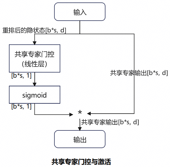

图4 共享专家门控与激活实现流程图

3.4 路由实现

实现专家路由的类是Qwen3_5MoeTopKRouter，其源码为

class Qwen3_5MoeTopKRouter(nn.Module):
    def __init__(self, config):
    super().__init__()
    self.top_k = config.num_experts_per_tok
    self.num_experts = config.num_experts
    self.hidden_dim = config.hidden_size
    self.weight = nn.Parameter(torch.zeros(self.num_experts, self.hidden_dim))

    def forward(self, hidden_states):
        hidden_states = hidden_states.reshape(-1, self.hidden_dim)
        router_logits = F.linear(hidden_states, self.weight)  # (seq_len, num_experts)
        router_probs = torch.nn.functional.softmax(router_logits, dtype=torch.float, dim=-1)
        router_top_value, router_indices = torch.topk(router_probs, self.top_k, dim=-1)  # (seq_len, top_k)
        router_top_value /= router_top_value.sum(dim=-1, keepdim=True)
        router_top_value = router_top_value.to(router_logits.dtype)
        router_scores = router_top_value
        return router_logits, router_scores, router_indices

计算流程如图5所示。输入隐藏状态经过线性变换和Softmax计算每个专家的概率分布，然后选取Top-K个专家并对权重进行归一化处理；最终返回原始logits、归一化后的专家权重以及对应索引。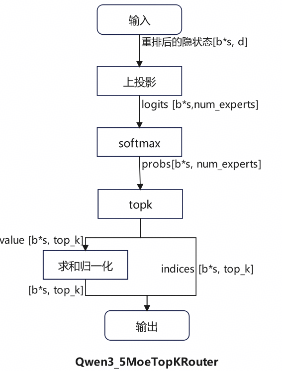

图5 Qwen3_5MoeTopKRouter 流程图

3.5 路由专家实现

实现路由专家的类是Qwen3_5MoeExperts，其源码为

@use_experts_implementation
class Qwen3_5MoeExperts(nn.Module):
    """Collection of expert weights stored as 3D tensors."""

    def __init__(self, config):
        super().__init__()
        self.num_experts = config.num_experts
        self.hidden_dim = config.hidden_size
        self.intermediate_dim = config.moe_intermediate_size
        self.gate_up_proj = nn.Parameter(torch.empty(self.num_experts, 2 * self.intermediate_dim, self.hidden_dim))
        self.down_proj = nn.Parameter(torch.empty(self.num_experts, self.hidden_dim, self.intermediate_dim))
        self.act_fn = ACT2FN[config.hidden_act]

    def forward(
        self,
        hidden_states: torch.Tensor,
        top_k_index: torch.Tensor,
        top_k_weights: torch.Tensor,
    ) -> torch.Tensor:
        final_hidden_states = torch.zeros_like(hidden_states)
        with torch.no_grad():
            expert_mask = torch.nn.functional.one_hot(top_k_index, num_classes=self.num_experts)
            expert_mask = expert_mask.permute(2, 1, 0)
            expert_hit = torch.greater(expert_mask.sum(dim=(-1, -2)), 0).nonzero()

        for expert_idx in expert_hit:
            expert_idx = expert_idx[0]
            if expert_idx == self.num_experts:
                continue
            top_k_pos, token_idx = torch.where(expert_mask[expert_idx])
            current_state = hidden_states[token_idx]
            gate, up = nn.functional.linear(current_state, self.gate_up_proj[expert_idx]).chunk(2, dim=-1)
            current_hidden_states = self.act_fn(gate) * up
            current_hidden_states = nn.functional.linear(current_hidden_states, self.down_proj[expert_idx])
            current_hidden_states = current_hidden_states * top_k_weights[token_idx, top_k_pos, None]
            final_hidden_states.index_add_(0, token_idx, current_hidden_states.to(final_hidden_states.dtype))

        return final_hidden_states

计算流程如图6所示。该模块首先根据路由输出的专家索引构建掩码，确定哪些专家被激活并获取对应的token位置；然后对每个被激活的专家，提取对应的隐藏状态，分别经过门控和上投影，将两者的计算结果传入激活函数进行计算得到激活值，再通过下投影和加权后，把结果累加到最终输出中。

图6 Qwen3_5MoeExperts 流程图

四、vLLM实现及关键算子

4.1 vLLM实现

Qwen3.5的MoE部分在vLLM中通过SharedFusedMoE类实现。在vLLM-ascend中，该类由AscendSharedFusedMoE代替。

AscendSharedFusedMoE.forward实现流程（源码链接：https://github.com/vllm-project/vllm-ascend/blob/main/vllm_ascend/ops/fused_moe/fused_moe.py#L549）

AscendSharedFusedMoE.forward()
->AscendFusedMoE.forward()
->AscendMoERunner.forward()
->AscendSharedFusedMoE.forward_impl()
->AscendFusedMoE.forward_impl() + AscendSharedFusedMoE._forward_shared_experts()
            路由专家                                   共享专家

AscendFusedMoE.forward_impl实现流程（假设不开启multistream_overlap_gate）（源码链接：https://github.com/vllm-project/vllm-ascend/blob/main/vllm_ascend/ops/fused_moe/fused_moe.py#L414）

准备阶段：_EXTRA_CTX.moe_comm_method.prepare()
专家计算：self.quant_method.apply()
如果开启了EPLB，计算每个专家处理的token数，更新负载统计信息，用于后续负载均衡优化
处理计算结果（规约、恢复形状等）：_EXTRA_CTX.moe_comm_method.finalize()

以w8a8量化类型为例来说明self.quant_method.apply的实现流程：此时quant_method=AscendW8A8DynamicFusedMoEMethod，进入AscendW8A8DynamicFusedMoEMethod.apply处理流程（源码链接：https://github.com/vllm-project/vllm-ascend/blob/main/vllm_ascend/quantization/methods/w8a8_dynamic.py#L109）

计算有效路由专家数量 valid_global_expert_num = global_num_experts - global_redundant_expert_num - n_shared_experts
获取路由权重和索引 topk_weights, topk_ids = select_experts()
获取路由专家融合输出 final_hidden_states = moe_comm_method.fused_experts

moe_comm_method.fused_experts实现流程（源码链接：vllm-ascend/vllm_ascend/ops/fused_moe/moe_comm_method.py at main · vllm-project/vllm-ascend (github.com)）

token分发
应用mlp计算路由专家输出
token结果聚合

AscendSharedFusedMoE._forward_shared_experts实现流程（源码链接：https://github.com/vllm-project/vllm-ascend/blob/main/vllm_ascend/ops/fused_moe/fused_moe.py#L683）

如果开启共享专家多流开关，切换到共享专家专用计算流
等待数据就绪
执行part1：门控投影+上投影
等待combine事件
执行part2：激活函数+下投影+门控与激活

4.2 关键算子

profliling算子名称	作用	对应接口	代码路径
MoeGatingTopK	MoE计算中，对输入x做Sigmoid或者SoftMax计算，对计算结果分组进行排序，最后根据分组排序的结果选取前k个专家	moe_gating_top_k	vllm-ascend/vllm_ascend/ops/fused_moe/experts_selector.py at main · vllm-project/vllm-ascend (github.com)
MoeInitRoutingCustom	根据aclnnMoeGatingTopKSoftmax的计算结果做routing处理	npu_moe_init_routing	vllm-ascend/vllm_ascend/ops/fused_moe/token_dispatcher.py at main · vllm-project/vllm-ascend (github.com)
GroupedMatmulSwigluQuant	融合GroupedMatmul、dquant、swiglu和quant	grouped_matmul_swiglu_quant_weight_nz_tensor_list	vllm-ascend/vllm_ascend/ops/fused_moe/moe_mlp.py at main · vllm-project/vllm-ascend (github.com)
GroupedMatmul	实现分组矩阵乘计算，每组矩阵乘的维度大小可以不同	npu_grouped_matmul	vllm-ascend/vllm_ascend/ops/fused_moe/moe_mlp.py at main · vllm-project/vllm-ascend (github.com)
MoeTokenUnpermute	根据sortedIndices存储的下标，获取permutedTokens中存储的输入数据；如果存在probs数据，permutedTokens会与probs相乘；最后进行累加求和，并输出计算结果	npu_moe_token_unpermute	vllm-ascend/vllm_ascend/ops/fused_moe/token_dispatcher.py at main · vllm-project/vllm-ascend (github.com)

五、profiling采集与分析

5.1 profiling采集

在服务化脚本中添加profiling采集参数，随后拉起服务。这里通过torch_profiler_dir指定profiling保存路径，torch_profiler_with_stack控制是否采集堆栈信息。由于采集堆栈信息会导致profiling文件膨胀，一般先关闭该开关。

--profiler-config '{"profiler": "torch", "torch_profiler_dir": "xxx", "torch_profiler_with_stack": false}' \

运行服务时，发送开始性能采集请求。

curl -X POST http://localhost:8113/start_profile

等待一定时间后，发送停止性能采集请求。

curl -X POST http://localhost:8113/stop_profile

对profiling做离线解析。通过profiler.analyse接口解析指定地址的profiling。这里的地址可以是前面指定的profiling存储目录，也可以指定到 xxx_ascend_pt 这一层。解析后的文件包含算子统计信息、算子详情等，且可被导入到Mindstudio Insight工具做进一步分析。

python3 -c "from torch_npu.profiler.profiler import analyse; analyse('xxx')"

5.2 profiling分析

5.2.1 MindStudio Insight界面介绍与prefill/decode界定

MindStudio Insight的时间线界面介绍见系统调优-MindStudio26.0.0-昇腾社区 (hiascend.com)。本profiling的时间线主要分为四部分：

• **Process xxx：host侧时间线。**包含多个线程的信息，每个线程下有pytorch和CANN的流水。
• **Ascend Hardware：device侧时间线。**包含多条流上的算子运算流水。
• **Communication：通信时间线。**包含本卡所在通信域下的通信算子信息与集合通信算子信息。
• **Overlap Analysis：总耗时占比时间线。**分为四个泳道，分别为Computing（计算时间）、Communication（通信时间）、Communication(Not Overlapped)（未被计算掩盖的通信时间）、Free（下发时间）。

对时间线界面有初步认知后，需要区分何处为prefill，何处为decode。
从执行顺序来看，prefill是整个推理过程中前部的大段连续计算；decode阶段是prefill之后的多次循环计算，每次decode对应一个token的生成，decode循环次数等于token生成数。故prefill是位于前部的一轮或多轮耗时较长的计算，而decode是紧接在prefill后面耗时较短的多轮重复计算。
从执行方式来看，prefill部分query的token数通常为多个，而decode部分query的token数为1个。因此prefill的注意力计算关键算子耗时会显著高于decode。
从算子层面来看，prefill从aclnnEmbedding开始，以aclnnArgMax结束；decode从MODEL_EXECUTE开始，以aclnnArgMax结束。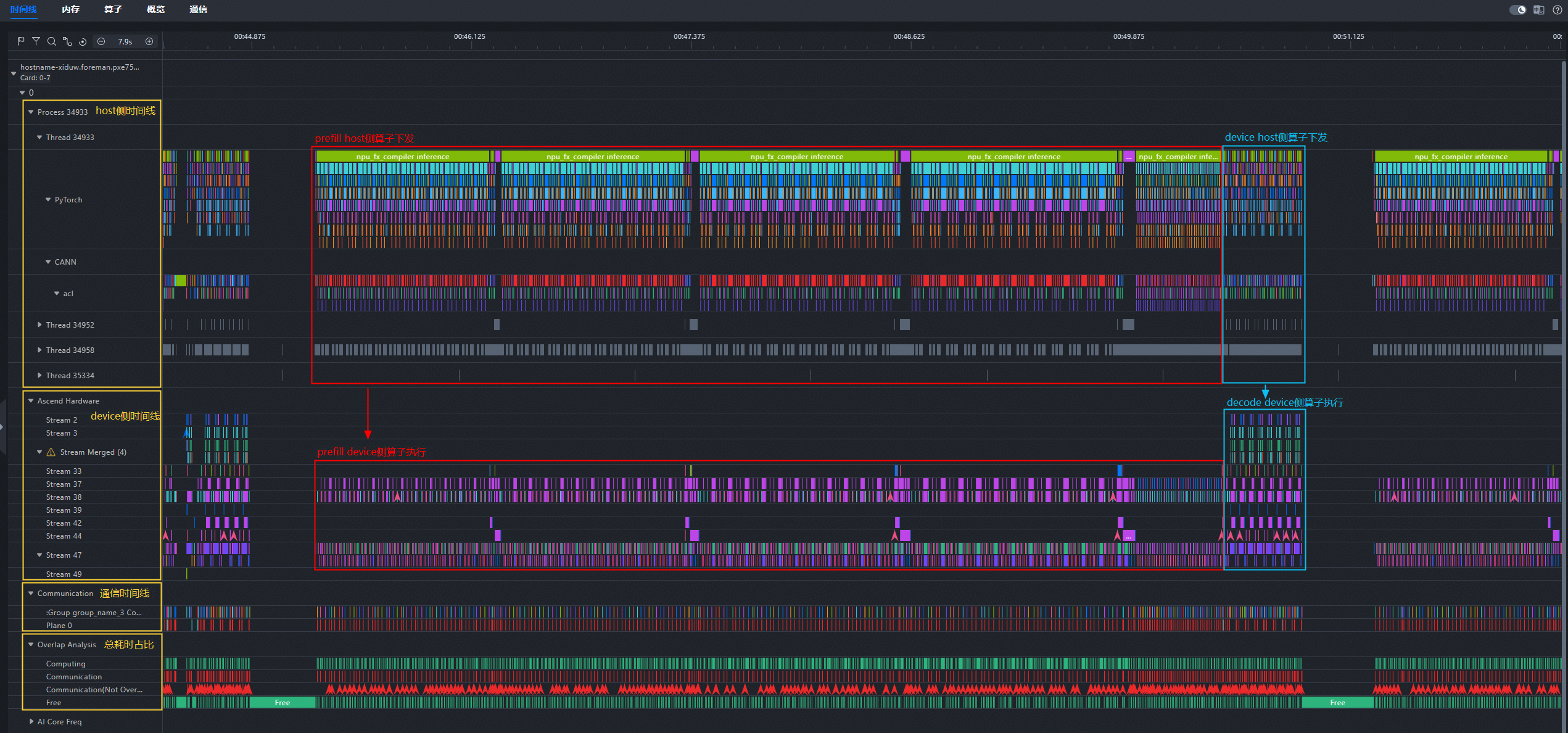

图7 prefill与decode界定示意图

5.2.2 单个decode拆解

当开启图模式时，一轮decode的开始算子为​aclnnInplaceFillScalar和MODEL_EXECUTE​，前者用于在自回归推理中执行​填充操作​，后者是acl graph成功开启的标志；结束算子为​aclnnArgMax​，用于在解码结束时选择输出概率最高的token​。
开启投机推理时，每轮decode会利用草稿模型多预测若干个token。​待主模型完成算子下发后，草稿模型开始下发算子。​在本profiling中，一轮decode内出现了4次aclnnArgMax，说明除主模型以外，草稿模型还预测了3个token。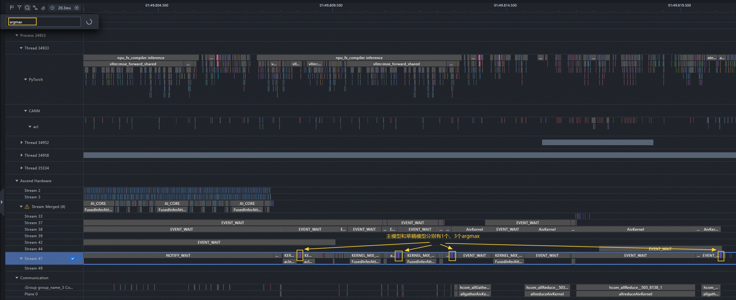

图8 单个decode中的主模型和草稿模型的argmax算子
明确device侧的主模型、草稿模型算子后，通过算子下发连线可以反推出主模型和草稿模型在host侧的位置。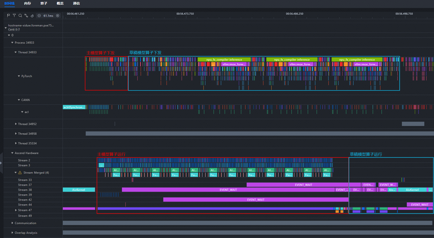

图9 划分主模型、草稿模型下发、计算部分

5.2.3 单层decode分析

结合模型结构对profiling进行拆解。观察图1中的模型结构，可以看到每个ResNet都以RMSNorm开始，故可以将RMSNorm算子作为界限来划分各个ResNet。这里取一段decode阶段的profiling，找到AddRmsNormBias后，从kernel_details.csv文件中找到后面两个AddRmsNormBias算子，复制这一段算子名称，得到的profiling信息如图10所示，对应的算子信息如表2所示。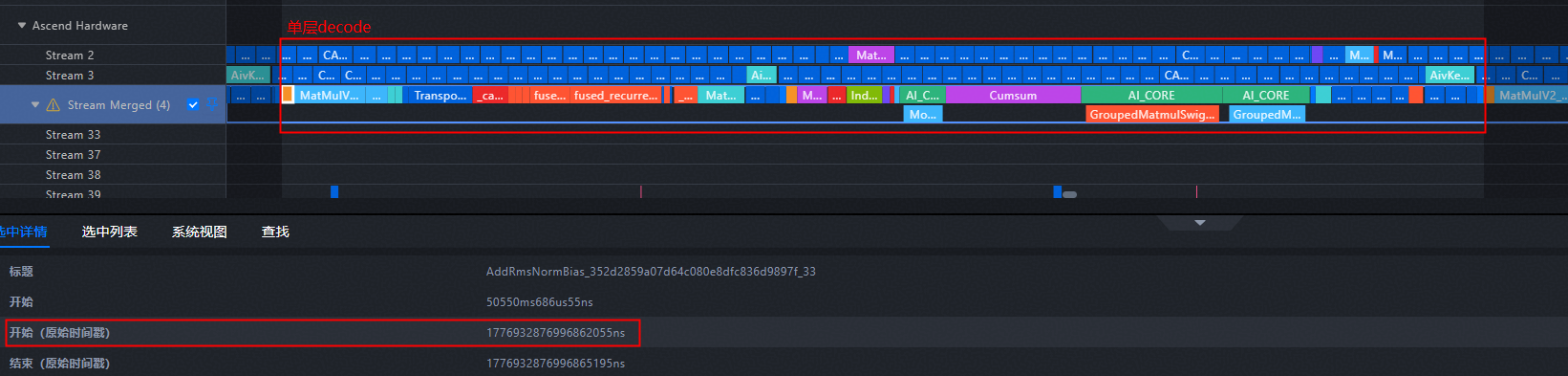

图10 decode阶段单层DecodeLayer profiling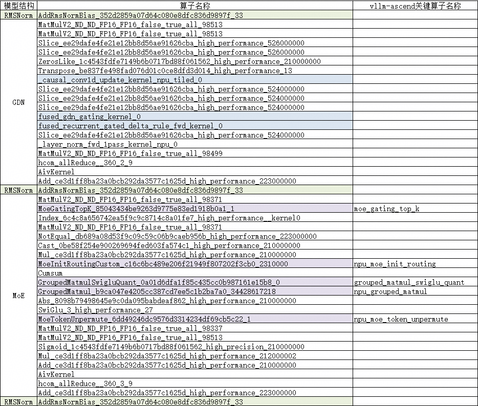

表2 decode阶段单层DecodeLayer算子汇总
观察到第一个ResNet包含_causal_conv1d_update_kernel_npu_tiled、fused_gdn_gating_kernel、fused_recurrent_gated_delta_rule_fwd_kernel等关键算子（表2中蓝色底纹标记部分），从而明确该部分在是GDN的实现。在第二个ResNet中包含MoeGatingTopK、MoeInitRoutingCustom、MoeTokenUnpermute等关键算子（表2中紫色底纹标记部分），可明确该部分在做MoE计算。