一、实验内容

1、论文阅读和视频学习

1.1 MobileNet V1&V2

• MobileNet_V1_V2⽹络讲解 https://www.bilibili.com/video/BV1yE411p7L7/
• Pytorch搭建MobileNetV2⽹络 （有余⼒的同学可学习代码）https://www.bilibili.com/video/BV1qE411T7qZ/

1.2 MobileNet V3

• MobileNet_V3⽹络讲解 https://www.bilibili.com/video/BV1GK4y1p7uE/
• Pytorch搭建MobileNetV3⽹络 （有余⼒的同学可学习代码） https://www.bilibili.com/video/BV1zT4y1P7pd/

1.3 ShuffleNet

• ShuffleNet ⽹络讲解 （ShuffleNetV1掌握就可以了，V2稍微了解下就好） https://www.bilibili.com/video/BV15y4y1Y7SY/
• 弄清楚 Channel 的 shuffle 是如何⽤代码实现的

1.4 SENet&CBAM

阅读Momenta公司的《ImageNet2017冠军模型-SENet详解》（访问链接），掌握SENet的基本原理。同时，学习SENet的示例代码（实验指导链接），数据加载和训练的代码可以参考ResNet（访问链接）

2. 代码作业

阅读论⽂《HybridSN: Exploring 3-D–2-DCNN Feature Hierarchy for Hyperspectral Image Classification》，思考3D卷积和2D卷积的区别。并阅读HybridSN的代码 (实验指导链接)

把代码敲⼊ Colab 运⾏，⽹络部分需要⾃⼰完成。

3D卷积和2D卷积的不同：

特性	2D 卷积	3D 卷积
卷积核形状	二维 (如 3×3)	三维 (如 3×3×3)
在HSI数据块上的移动方式	仅沿高度和宽度滑动	沿高度、宽度和光谱波段滑动
特征焦点	空间特征 (一次性处理所有波段)	空谱联合特征 (从局部3D数据块中学习)
优点	计算高效，不易过拟合	特征提取能力强，能很好地为光谱关系建模
缺点	无法显式学习波段间的相关性	计算成本高，参数多，更容易过拟合
在HybridSN中的作用	在网络后端，学习深层、抽象的空间特征	在网络前端，提取基础且关键的空谱联合特征

这篇论文构建了一个混合网络解决高光谱图像分类问题，首先用3D卷积，然后使用2D卷积，代码相对简单，下面是代码的解析。

首先取得数据，并引入基本函数库。

! wget http://www.ehu.eus/ccwintco/uploads/6/67/Indian_pines_corrected.mat
! wget http://www.ehu.eus/ccwintco/uploads/c/c4/Indian_pines_gt.mat
! pip install spectral

import numpy as np
import matplotlib.pyplot as plt
import scipy.io as sio
from sklearn.decomposition import PCA
from sklearn.model_selection import train_test_split
from sklearn.metrics import confusion_matrix, accuracy_score, classification_report, cohen_kappa_score
import spectral
import torch
import torchvision
import torch.nn as nn
import torch.nn.functional as F
import torch.optim as optim

2.1. 定义HybridSN类

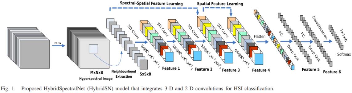
模型的网络结构如下图所示：

三维卷积部分：

• conv1：（1, 30, 25, 25）， 8个 7x3x3 的卷积核 ==>（8, 24, 23, 23）
• conv2：（8, 24, 23, 23）， 16个 5x3x3 的卷积核 ==>（16, 20, 21, 21）
• conv3：（16, 20, 21, 21），32个 3x3x3 的卷积核 ==>（32, 18, 19, 19）

接下来要进行二维卷积，因此吧前面的$32\ast 18$reshape一下，得到了$(576,19,19)$

二维卷积：$（576,19,19）$ 64个 $3*3 $的卷积核，得到 $(64,17,17)$

接下来是一个 flatten 操作，变为 18496 维的向量，

接下来依次为256，128节点的全连接层，都使用比例为0.4的 Dropout，

最后输出为 16 个节点，是最终的分类类别数。

下面是 HybridSN 类的代码：

import torch
import torch.nn as nn

class_num = 16

class HybridSN(nn.Module):
    """
    HybridSN: A Hybrid Spectral-Spatial Network for Hyperspectral Image Classification
    """
    def __init__(self, num_classes=16):
        super(HybridSN, self).__init__()
        # 3D 卷积层
        self.conv3d_1 = nn.Sequential(
            nn.Conv3d(1, 8, kernel_size=(7, 3, 3), stride=1, padding=0),
            nn.ReLU(inplace=True)
        )
        self.conv3d_2 = nn.Sequential(
            nn.Conv3d(8, 16, kernel_size=(5, 3, 3), stride=1, padding=0),
            nn.ReLU(inplace=True)
        )
        self.conv3d_3 = nn.Sequential(
            nn.Conv3d(16, 32, kernel_size=(3, 3, 3), stride=1, padding=0),
            nn.ReLU(inplace=True)
        )

        # 2D 卷积层
        self.conv2d_1 = nn.Sequential(
            # 输入通道数为 32 * 18 = 576
            nn.Conv2d(576, 64, kernel_size=(3, 3), stride=1, padding=0),
            nn.ReLU(inplace=True)
        )

        # 全连接层
        self.fc1 = nn.Sequential(
            # 输入维度为 64 * 17 * 17 = 18496
            nn.Linear(18496, 256),
            nn.ReLU(inplace=True),
            nn.Dropout(0.4)   #这里使用了暂退法，并且没有区分train和test，可以加个参数来区分一下
        )
        self.fc2 = nn.Sequential(
            nn.Linear(256, 128),
            nn.ReLU(inplace=True),
            nn.Dropout(0.4)   #这里同上
        )
        self.fc3 = nn.Linear(128, num_classes)

    def forward(self, x):
        # 预期输入 x 的形状: (batch_size, 1, 30, 25, 25)
        # 注意：PyTorch 的 Conv3d 需要一个通道维度，所以输入应该是 (N, C_in, D, H, W)
        # 原始描述 (1, 30, 25, 25) 缺少批量维度 N，我们假设为 (N, 1, 30, 25, 25)

        # 3D 卷积部分
        out = self.conv3d_1(x)
        out = self.conv3d_2(out)
        out = self.conv3d_3(out)

        # Reshape 操作
        # out.shape: (N, 32, 18, 19, 19)
        # 重塑为: (N, 576, 19, 19)
        out = out.view(out.size(0), -1, out.size(3), out.size(4))

        # 2D 卷积部分
        out = self.conv2d_1(out)

        # Flatten 操作
        # out.shape: (N, 64, 17, 17)
        # 展平为: (N, 18496)
        out = out.view(out.size(0), -1)

        # 全连接分类部分
        out = self.fc1(out)
        out = self.fc2(out)
        out = self.fc3(out)

        return out

# 随机输入，测试网络结构是否通畅
# 输入形状应为 (批量大小, 通道数, 光谱带数, 高, 宽)
# 对应描述中的 (1, 30, 25, 25)，我们需要在前面加上批量大小和通道数
x = torch.randn(1, 1, 30, 25, 25)
net = HybridSN(num_classes=class_num)
y = net(x)
print(y.shape) # 预期输出: torch.Size([1, 16])

输出如下：

torch.Size([1, 16])

2.2、定义数据集

首先对高光谱数据实施PCA降维；然后创建 keras 方便处理的数据格式；然后随机抽取 10% 数据做为训练集，剩余的做为测试集。

首先定义基本函数

# 对高光谱数据 X 应用 PCA 变换
def applyPCA(X, numComponents):
    newX = np.reshape(X, (-1, X.shape[2]))
    pca = PCA(n_components=numComponents, whiten=True)
    newX = pca.fit_transform(newX)
    newX = np.reshape(newX, (X.shape[0], X.shape[1], numComponents))
    return newX

# 对单个像素周围提取 patch 时，边缘像素就无法取了，因此，给这部分像素进行 padding 操作
def padWithZeros(X, margin=2):
    newX = np.zeros((X.shape[0] + 2 * margin, X.shape[1] + 2* margin, X.shape[2]))
    x_offset = margin
    y_offset = margin
    newX[x_offset:X.shape[0] + x_offset, y_offset:X.shape[1] + y_offset, :] = X
    return newX

# 在每个像素周围提取 patch ，然后创建成符合 keras 处理的格式
def createImageCubes(X, y, windowSize=5, removeZeroLabels = True):
    # 给 X 做 padding
    margin = int((windowSize - 1) / 2)
    zeroPaddedX = padWithZeros(X, margin=margin)
    # split patches
    patchesData = np.zeros((X.shape[0] * X.shape[1], windowSize, windowSize, X.shape[2]))
    patchesLabels = np.zeros((X.shape[0] * X.shape[1]))
    patchIndex = 0
    for r in range(margin, zeroPaddedX.shape[0] - margin):
        for c in range(margin, zeroPaddedX.shape[1] - margin):
            patch = zeroPaddedX[r - margin:r + margin + 1, c - margin:c + margin + 1]   
            patchesData[patchIndex, :, :, :] = patch
            patchesLabels[patchIndex] = y[r-margin, c-margin]
            patchIndex = patchIndex + 1
    if removeZeroLabels:
        patchesData = patchesData[patchesLabels>0,:,:,:]
        patchesLabels = patchesLabels[patchesLabels>0]
        patchesLabels -= 1
    return patchesData, patchesLabels

def splitTrainTestSet(X, y, testRatio, randomState=345):
    X_train, X_test, y_train, y_test = train_test_split(X, y, test_size=testRatio, random_state=randomState, stratify=y)
    return X_train, X_test, y_train, y_test

接下来读取并创建数据集：

# 地物类别
class_num = 16
X = sio.loadmat('Indian_pines_corrected.mat')['indian_pines_corrected']
y = sio.loadmat('Indian_pines_gt.mat')['indian_pines_gt']

# 用于测试样本的比例
test_ratio = 0.90
# 每个像素周围提取 patch 的尺寸
patch_size = 25
# 使用 PCA 降维，得到主成分的数量
pca_components = 30

print('Hyperspectral data shape: ', X.shape)
print('Label shape: ', y.shape)

print('\n... ... PCA tranformation ... ...')
X_pca = applyPCA(X, numComponents=pca_components)
print('Data shape after PCA: ', X_pca.shape)

print('\n... ... create data cubes ... ...')
X_pca, y = createImageCubes(X_pca, y, windowSize=patch_size)
print('Data cube X shape: ', X_pca.shape)
print('Data cube y shape: ', y.shape)

print('\n... ... create train & test data ... ...')
Xtrain, Xtest, ytrain, ytest = splitTrainTestSet(X_pca, y, test_ratio)
print('Xtrain shape: ', Xtrain.shape)
print('Xtest  shape: ', Xtest.shape)

# 改变 Xtrain, Ytrain 的形状，以符合 keras 的要求
Xtrain = Xtrain.reshape(-1, patch_size, patch_size, pca_components, 1)
Xtest  = Xtest.reshape(-1, patch_size, patch_size, pca_components, 1)
print('before transpose: Xtrain shape: ', Xtrain.shape) 
print('before transpose: Xtest  shape: ', Xtest.shape) 

# 为了适应 pytorch 结构，数据要做 transpose
Xtrain = Xtrain.transpose(0, 4, 3, 1, 2)
Xtest  = Xtest.transpose(0, 4, 3, 1, 2)
print('after transpose: Xtrain shape: ', Xtrain.shape) 
print('after transpose: Xtest  shape: ', Xtest.shape) 


""" Training dataset"""
class TrainDS(torch.utils.data.Dataset): 
    def __init__(self):
        self.len = Xtrain.shape[0]
        self.x_data = torch.FloatTensor(Xtrain)
        self.y_data = torch.LongTensor(ytrain)        
    def __getitem__(self, index):
        # 根据索引返回数据和对应的标签
        return self.x_data[index], self.y_data[index]
    def __len__(self): 
        # 返回文件数据的数目
        return self.len

""" Testing dataset"""
class TestDS(torch.utils.data.Dataset): 
    def __init__(self):
        self.len = Xtest.shape[0]
        self.x_data = torch.FloatTensor(Xtest)
        self.y_data = torch.LongTensor(ytest)
    def __getitem__(self, index):
        # 根据索引返回数据和对应的标签
        return self.x_data[index], self.y_data[index]
    def __len__(self): 
        # 返回文件数据的数目
        return self.len

# 创建 trainloader 和 testloader
trainset = TrainDS()
testset  = TestDS()
train_loader = torch.utils.data.DataLoader(dataset=trainset, batch_size=128, shuffle=True, num_workers=2)
test_loader  = torch.utils.data.DataLoader(dataset=testset,  batch_size=128, shuffle=False, num_workers=2)

输出如下：

Hyperspectral data shape:  (145, 145, 200)
Label shape:  (145, 145)

... ... PCA tranformation ... ...
Data shape after PCA:  (145, 145, 30)

... ... create data cubes ... ...
Data cube X shape:  (10249, 25, 25, 30)
Data cube y shape:  (10249,)

... ... create train & test data ... ...
Xtrain shape:  (1024, 25, 25, 30)
Xtest  shape:  (9225, 25, 25, 30)
before transpose: Xtrain shape:  (1024, 25, 25, 30, 1)
before transpose: Xtest  shape:  (9225, 25, 25, 30, 1)
after transpose: Xtrain shape:  (1024, 1, 30, 25, 25)
after transpose: Xtest  shape:  (9225, 1, 30, 25, 25)

2.3、开始训练

# 使用GPU训练，可以在菜单 "代码执行工具" -> "更改运行时类型" 里进行设置
device = torch.device("cuda:0" if torch.cuda.is_available() else "cpu")

# 网络放到GPU上
net = HybridSN().to(device)
criterion = nn.CrossEntropyLoss()
optimizer = optim.Adam(net.parameters(), lr=0.001)

# 开始训练
total_loss = 0
for epoch in range(100):
    for i, (inputs, labels) in enumerate(train_loader):
        inputs = inputs.to(device)
        labels = labels.to(device)
        # 优化器梯度归零
        optimizer.zero_grad()
        # 正向传播 +　反向传播 + 优化 
        outputs = net(inputs)
        loss = criterion(outputs, labels)
        loss.backward()
        optimizer.step()
        total_loss += loss.item()
    print('[Epoch: %d]   [loss avg: %.4f]   [current loss: %.4f]' %(epoch + 1, total_loss/(epoch+1), loss.item()))

print('Finished Training')

输出如下：

[Epoch: 1]   [loss avg: 21.9907]   [current loss: 2.6568]
[Epoch: 2]   [loss avg: 21.7384]   [current loss: 2.7878]
[Epoch: 3]   [loss avg: 21.2243]   [current loss: 2.4659]
[Epoch: 4]   [loss avg: 20.7703]   [current loss: 2.4362]
[Epoch: 5]   [loss avg: 20.3855]   [current loss: 2.3429]
[Epoch: 6]   [loss avg: 20.0578]   [current loss: 2.4317]
[Epoch: 7]   [loss avg: 19.7465]   [current loss: 2.1637]
[Epoch: 8]   [loss avg: 19.4192]   [current loss: 2.0932]
[Epoch: 9]   [loss avg: 19.1249]   [current loss: 2.2235]
[Epoch: 10]   [loss avg: 18.8745]   [current loss: 2.0129]
[Epoch: 11]   [loss avg: 18.6103]   [current loss: 1.9912]
[Epoch: 12]   [loss avg: 18.3366]   [current loss: 1.8624]
[Epoch: 13]   [loss avg: 18.0223]   [current loss: 1.7838]
[Epoch: 14]   [loss avg: 17.6630]   [current loss: 1.6799]
[Epoch: 15]   [loss avg: 17.2822]   [current loss: 1.3895]
[Epoch: 16]   [loss avg: 16.8884]   [current loss: 1.4154]
[Epoch: 17]   [loss avg: 16.4715]   [current loss: 1.2353]
[Epoch: 18]   [loss avg: 16.0531]   [current loss: 0.9989]
[Epoch: 19]   [loss avg: 15.6341]   [current loss: 1.0417]
[Epoch: 20]   [loss avg: 15.2127]   [current loss: 0.8861]
[Epoch: 21]   [loss avg: 14.7777]   [current loss: 0.6804]
[Epoch: 22]   [loss avg: 14.3331]   [current loss: 0.6048]
[Epoch: 23]   [loss avg: 13.8949]   [current loss: 0.5720]
[Epoch: 24]   [loss avg: 13.4768]   [current loss: 0.3803]
[Epoch: 25]   [loss avg: 13.0599]   [current loss: 0.4180]
[Epoch: 26]   [loss avg: 12.6624]   [current loss: 0.3007]
[Epoch: 27]   [loss avg: 12.2748]   [current loss: 0.2992]
[Epoch: 28]   [loss avg: 11.9072]   [current loss: 0.2700]
[Epoch: 29]   [loss avg: 11.5576]   [current loss: 0.2123]
[Epoch: 30]   [loss avg: 11.2133]   [current loss: 0.2440]
[Epoch: 31]   [loss avg: 10.8867]   [current loss: 0.1662]
[Epoch: 32]   [loss avg: 10.5782]   [current loss: 0.1632]
[Epoch: 33]   [loss avg: 10.2794]   [current loss: 0.0692]
[Epoch: 34]   [loss avg: 9.9976]   [current loss: 0.0588]
[Epoch: 35]   [loss avg: 9.7291]   [current loss: 0.0292]
[Epoch: 36]   [loss avg: 9.4784]   [current loss: 0.1100]
[Epoch: 37]   [loss avg: 9.2378]   [current loss: 0.1004]
[Epoch: 38]   [loss avg: 9.0063]   [current loss: 0.0279]
[Epoch: 39]   [loss avg: 8.7908]   [current loss: 0.1023]
[Epoch: 40]   [loss avg: 8.5885]   [current loss: 0.0201]
[Epoch: 41]   [loss avg: 8.3997]   [current loss: 0.1805]
[Epoch: 42]   [loss avg: 8.2137]   [current loss: 0.0785]
[Epoch: 43]   [loss avg: 8.0333]   [current loss: 0.0274]
[Epoch: 44]   [loss avg: 7.8639]   [current loss: 0.0785]
[Epoch: 45]   [loss avg: 7.7058]   [current loss: 0.0702]
[Epoch: 46]   [loss avg: 7.5498]   [current loss: 0.0739]
[Epoch: 47]   [loss avg: 7.3998]   [current loss: 0.0833]
[Epoch: 48]   [loss avg: 7.2587]   [current loss: 0.1817]
[Epoch: 49]   [loss avg: 7.1184]   [current loss: 0.0328]
[Epoch: 50]   [loss avg: 6.9843]   [current loss: 0.1010]
[Epoch: 51]   [loss avg: 6.8605]   [current loss: 0.1132]
[Epoch: 52]   [loss avg: 6.7369]   [current loss: 0.0607]
[Epoch: 53]   [loss avg: 6.6170]   [current loss: 0.0515]
[Epoch: 54]   [loss avg: 6.5028]   [current loss: 0.1119]
[Epoch: 55]   [loss avg: 6.3908]   [current loss: 0.0322]
[Epoch: 56]   [loss avg: 6.2819]   [current loss: 0.0229]
[Epoch: 57]   [loss avg: 6.1757]   [current loss: 0.0435]
[Epoch: 58]   [loss avg: 6.0731]   [current loss: 0.0564]
[Epoch: 59]   [loss avg: 5.9735]   [current loss: 0.0367]
[Epoch: 60]   [loss avg: 5.8765]   [current loss: 0.0146]
[Epoch: 61]   [loss avg: 5.7843]   [current loss: 0.0038]
[Epoch: 62]   [loss avg: 5.6930]   [current loss: 0.0294]
[Epoch: 63]   [loss avg: 5.6047]   [current loss: 0.0073]
[Epoch: 64]   [loss avg: 5.5211]   [current loss: 0.0102]
[Epoch: 65]   [loss avg: 5.4393]   [current loss: 0.0282]
[Epoch: 66]   [loss avg: 5.3597]   [current loss: 0.0194]
[Epoch: 67]   [loss avg: 5.2818]   [current loss: 0.0112]
[Epoch: 68]   [loss avg: 5.2079]   [current loss: 0.0079]
[Epoch: 69]   [loss avg: 5.1379]   [current loss: 0.0454]
[Epoch: 70]   [loss avg: 5.0676]   [current loss: 0.0457]
[Epoch: 71]   [loss avg: 4.9993]   [current loss: 0.0072]
[Epoch: 72]   [loss avg: 4.9319]   [current loss: 0.0038]
[Epoch: 73]   [loss avg: 4.8665]   [current loss: 0.0032]
[Epoch: 74]   [loss avg: 4.8022]   [current loss: 0.0056]
[Epoch: 75]   [loss avg: 4.7411]   [current loss: 0.0018]
[Epoch: 76]   [loss avg: 4.6804]   [current loss: 0.0027]
[Epoch: 77]   [loss avg: 4.6227]   [current loss: 0.0144]
[Epoch: 78]   [loss avg: 4.5675]   [current loss: 0.1498]
[Epoch: 79]   [loss avg: 4.5123]   [current loss: 0.0660]
[Epoch: 80]   [loss avg: 4.4585]   [current loss: 0.0028]
[Epoch: 81]   [loss avg: 4.4049]   [current loss: 0.0043]
[Epoch: 82]   [loss avg: 4.3522]   [current loss: 0.0093]
[Epoch: 83]   [loss avg: 4.3004]   [current loss: 0.0018]
[Epoch: 84]   [loss avg: 4.2505]   [current loss: 0.0025]
[Epoch: 85]   [loss avg: 4.2027]   [current loss: 0.0196]
[Epoch: 86]   [loss avg: 4.1560]   [current loss: 0.0046]
[Epoch: 87]   [loss avg: 4.1102]   [current loss: 0.0518]
[Epoch: 88]   [loss avg: 4.0668]   [current loss: 0.1038]
[Epoch: 89]   [loss avg: 4.0225]   [current loss: 0.0149]
[Epoch: 90]   [loss avg: 3.9792]   [current loss: 0.0401]
[Epoch: 91]   [loss avg: 3.9373]   [current loss: 0.0435]
[Epoch: 92]   [loss avg: 3.8958]   [current loss: 0.0228]
[Epoch: 93]   [loss avg: 3.8575]   [current loss: 0.0048]
[Epoch: 94]   [loss avg: 3.8177]   [current loss: 0.0130]
[Epoch: 95]   [loss avg: 3.7790]   [current loss: 0.0320]
[Epoch: 96]   [loss avg: 3.7404]   [current loss: 0.0227]
[Epoch: 97]   [loss avg: 3.7031]   [current loss: 0.0022]
[Epoch: 98]   [loss avg: 3.6664]   [current loss: 0.0086]
[Epoch: 99]   [loss avg: 3.6310]   [current loss: 0.0062]
[Epoch: 100]   [loss avg: 3.5957]   [current loss: 0.0151]
Finished Training

2.4、模型测试

count = 0
# 模型测试
for inputs, _ in test_loader:
    inputs = inputs.to(device)
    outputs = net(inputs)
    outputs = np.argmax(outputs.detach().cpu().numpy(), axis=1)
    if count == 0:
        y_pred_test =  outputs
        count = 1
    else:
        y_pred_test = np.concatenate( (y_pred_test, outputs) )

# 生成分类报告
classification = classification_report(ytest, y_pred_test, digits=4)
print(classification)

输出如下：

              precision    recall  f1-score   support

         0.0     0.9615    0.6098    0.7463        41
         1.0     0.9811    0.9276    0.9536      1285
         2.0     0.9175    0.9679    0.9420       747
         3.0     0.8843    0.8967    0.8904       213
         4.0     0.9362    0.9448    0.9405       435
         5.0     0.9816    0.9726    0.9771       657
         6.0     0.7667    0.9200    0.8364        25
         7.0     0.9572    0.9372    0.9471       430
         8.0     0.7000    0.7778    0.7368        18
         9.0     0.9391    0.9520    0.9455       875
        10.0     0.9703    0.9747    0.9725      2210
        11.0     0.8895    0.8895    0.8895       534
        12.0     0.9489    0.9027    0.9252       185
        13.0     0.9626    0.9956    0.9789      1139
        14.0     0.8992    0.9251    0.9119       347
        15.0     0.7910    0.6310    0.7020        84

    accuracy                         0.9494      9225
   macro avg     0.9054    0.8891    0.8935      9225
weighted avg     0.9497    0.9494    0.9490      9225

这里我们看到说准确率为94.94%，性能还是可以的。

2.5、备用函数

from operator import truediv

def AA_andEachClassAccuracy(confusion_matrix):
    counter = confusion_matrix.shape[0]
    list_diag = np.diag(confusion_matrix)
    list_raw_sum = np.sum(confusion_matrix, axis=1)
    each_acc = np.nan_to_num(truediv(list_diag, list_raw_sum))
    average_acc = np.mean(each_acc)
    return each_acc, average_acc


def reports (test_loader, y_test, name):
    count = 0
    # 模型测试
    for inputs, _ in test_loader:
        inputs = inputs.to(device)
        outputs = net(inputs)
        outputs = np.argmax(outputs.detach().cpu().numpy(), axis=1)
        if count == 0:
            y_pred =  outputs
            count = 1
        else:
            y_pred = np.concatenate( (y_pred, outputs) )

    if name == 'IP':
        target_names = ['Alfalfa', 'Corn-notill', 'Corn-mintill', 'Corn'
                        ,'Grass-pasture', 'Grass-trees', 'Grass-pasture-mowed', 
                        'Hay-windrowed', 'Oats', 'Soybean-notill', 'Soybean-mintill',
                        'Soybean-clean', 'Wheat', 'Woods', 'Buildings-Grass-Trees-Drives',
                        'Stone-Steel-Towers']
    elif name == 'SA':
        target_names = ['Brocoli_green_weeds_1','Brocoli_green_weeds_2','Fallow','Fallow_rough_plow','Fallow_smooth',
                        'Stubble','Celery','Grapes_untrained','Soil_vinyard_develop','Corn_senesced_green_weeds',
                        'Lettuce_romaine_4wk','Lettuce_romaine_5wk','Lettuce_romaine_6wk','Lettuce_romaine_7wk',
                        'Vinyard_untrained','Vinyard_vertical_trellis']
    elif name == 'PU':
        target_names = ['Asphalt','Meadows','Gravel','Trees', 'Painted metal sheets','Bare Soil','Bitumen',
                        'Self-Blocking Bricks','Shadows']
    
    classification = classification_report(y_test, y_pred, target_names=target_names)
    oa = accuracy_score(y_test, y_pred)
    confusion = confusion_matrix(y_test, y_pred)
    each_acc, aa = AA_andEachClassAccuracy(confusion)
    kappa = cohen_kappa_score(y_test, y_pred)
    
    return classification, confusion, oa*100, each_acc*100, aa*100, kappa*100

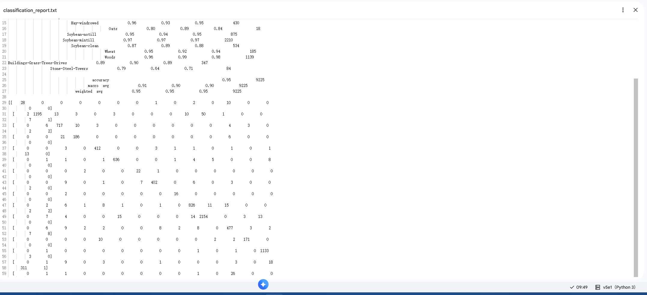
测试结果写在文件中：

classification, confusion, oa, each_acc, aa, kappa = reports(test_loader, ytest, 'IP')
classification = str(classification)
confusion = str(confusion)
file_name = "classification_report.txt"

with open(file_name, 'w') as x_file:
    x_file.write('\n')
    x_file.write('{} Kappa accuracy (%)'.format(kappa))
    x_file.write('\n')
    x_file.write('{} Overall accuracy (%)'.format(oa))
    x_file.write('\n')
    x_file.write('{} Average accuracy (%)'.format(aa))
    x_file.write('\n')
    x_file.write('\n')
    x_file.write('{}'.format(classification))
    x_file.write('\n')
    x_file.write('{}'.format(confusion))

结果如下：

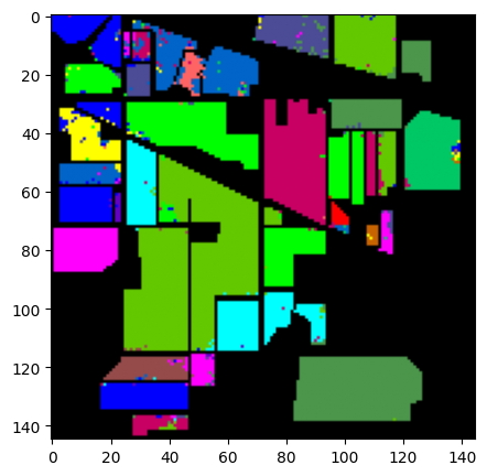
下面的代码用于显示分类结果：

# load the original image
X = sio.loadmat('Indian_pines_corrected.mat')['indian_pines_corrected']
y = sio.loadmat('Indian_pines_gt.mat')['indian_pines_gt']

height = y.shape[0]
width = y.shape[1]

X = applyPCA(X, numComponents= pca_components)
X = padWithZeros(X, patch_size//2)

# 逐像素预测类别
outputs = np.zeros((height,width))
for i in range(height):
    for j in range(width):
        if int(y[i,j]) == 0:
            continue
        else :
            image_patch = X[i:i+patch_size, j:j+patch_size, :]
            image_patch = image_patch.reshape(1,image_patch.shape[0],image_patch.shape[1], image_patch.shape[2], 1)
            X_test_image = torch.FloatTensor(image_patch.transpose(0, 4, 3, 1, 2)).to(device)                                   
            prediction = net(X_test_image)
            prediction = np.argmax(prediction.detach().cpu().numpy(), axis=1)
            outputs[i][j] = prediction+1
    if i % 20 == 0:
        print('... ... row ', i, ' handling ... ...')

输出如下：

/tmp/ipython-input-1433302639.py:23: DeprecationWarning: Conversion of an array with ndim > 0 to a scalar is deprecated, and will error in future. Ensure you extract a single element from your array before performing this operation. (Deprecated NumPy 1.25.)
  outputs[i][j] = prediction+1
... ... row  0  handling ... ...
... ... row  20  handling ... ...
... ... row  40  handling ... ...
... ... row  60  handling ... ...
... ... row  80  handling ... ...
... ... row  100  handling ... ...
... ... row  120  handling ... ...
... ... row  140  handling ... ...

predict_image = spectral.imshow(classes = outputs.astype(int),figsize =(5,5))

二、问题总结与体会

描述实验过程中所遇到的问题，以及是如何解决的。有哪些收获和体会，对于课程的安排有哪些建议。

● 训练HybridSN，然后多测试⼏次，会发现每次分类的结果都不⼀样，请思考为什么？

虽然模型训练好了之后就应该固定但是因为我们在网络中使用了DropOut，并且没有区分train和test，所以训练的时候会随机丢弃一些节点，这就会使得我们的结果不是很稳定。

● 如果想要进⼀步提升⾼光谱图像的分类性能，可以如何改进？

1. 在数据层面，本次实验中测试集的比例为train_ratio=0.90，意味着我们只用了10%的数据进行训练。这是导致我们性能受限的主要原因。同时我们还可以对我们的训练数据进行随机的旋转、翻转、添加高斯噪声等操作来增强模型的泛化能力。
2. 随着技术的发展，我们可以使用更加先进的网络模块，比如引入残差连接、注意力机制等。
3. 同时也可以调整一下我们的超参数。

● depth-wise conv 和 分组卷积有什么区别与联系？

1. 分组卷积:

   它的机制是将输入的 C 个通道分成 g 个组，每个组有 C/g 个通道。然后，卷积核也被分成 g 组，每一组卷积核只对相应的一组输入通道进行卷积操作。最后将 g 组的结果拼接起来。最初是为了在有限的硬件资源（如多个GPU）上训练大模型（如AlexNet）。现在主要用于减少参数量和计算量，构建更高效的网络（如ResNeXt）。

2. depth_wise:

   这是分组卷积在 g = C（分组数等于输入通道数）时的特殊情况。这意味着每一个卷积核只负责处理一个输入通道。它只在空间维度上进行滤波，完全不涉及通道之间的信息融合。 它的核心作用是分离空间卷积和通道卷积。因此，它通常会与一个逐点卷积 (Pointwise Convolution)，即1x1的普通卷积，组合使用。Depth-wise conv 负责空间特征提取，Pointwise conv 负责通道信息融合。这个组合（Depth-wise + Pointwise）就是 深度可分离卷积块 (Depthwise Separable Convolution)，是 MobileNet 系列网络的核心。

● SENet 的注意⼒是不是可以加在空间位置上？

应该是可以的，现在有其他的研究实现了这一点，比如CBAM，Block Attention Module。

● 在 ShuffleNet 中，通道的 shuffle 如何⽤代码实现？

通过 view 操作将通道维度“展开”成组的维度，然后通过 transpose 将这些组进行“交叉”，最后再通过 view 操作“压平”回去，就巧妙地完成了通道的混洗。

def channel_shuffle(x, groups):
    batch_size, num_channels, height, width = x.size()
    channels_per_group = num_channels // groups
    x = x.view(batch_size, groups, channels_per_group, height, width)
    x = x.transpose(1, 2).contiguous()
    x = x.view(batch_size, -1, height, width)
    return x

import torch
input_tensor = torch.randn(1, 4, 3, 3) # (N, C, H, W)
shuffled_tensor = channel_shuffle(input_tensor, groups=2)
print("Original shape:", input_tensor.shape)
print("Shuffled shape:", shuffled_tensor.shape)

体会：

在本次实验中我深入的学习了多种轻量级卷积神经网络，并亲手实践了HybridSN模型。在学习MobileNet和shuffleNet的过程中，我很深刻的看到了计算机工程师们是如何利用更少的资源去达到一个相对来说优的结果，用大概$1/8$的计算量就达到了基本相当的准确率。其次就是说SENet的通道注意力机制，让模型像人一样有重点的去关注信息，这让我想到了之前实验中的残差。此外就是暂退法，这个我之前也有接触过，老师上课也有讲过，test和train过程中dropout的效果，但是这大概是我第一次如此直观的看到。

但是还是有很多的问题，可能由于软工方面对神经网络这方面的关注较少，课程较少，所以导致说这其中的大多说代码我都是连蒙带猜加ai才能稍微明白是个什么意思。对于各种网络我也始终是镜中花水中月，总是不真切，可能需要更加系统的学习才行。