引言：为什么RNN是时序数据的"救世主"？

想象你在看一部电影，当主角说出"我觉得…“时，你能猜到下一句可能是"我们应该放弃"还是"这事儿有戏”——这依赖于你对前文剧情的记忆。现实世界中，电力负荷、股票价格、气象数据都是这样的"连续剧"，而循环神经网络（RNN）就是能"记住前文"的AI观众。

本文将带你吃透8种RNN变体（从基础到魔改），用一个电力负荷预测实战项目告诉你：为什么LSTM能解决"遗忘症"？双向模型如何"未卜先知"？Peephole LSTM的"偷看"技巧有多秀？最后用代码证明：哪种模型能让电网调度中心的预测误差跌破5%！

另外我整理了RNN相关资料包，感兴趣的可以自取，希望能帮到你！

原文 资料 这里！

一、通俗理解：RNN家族的"性格说明书"

1. 基础RNN：记性差的"鱼"

基础RNN就像只有7秒记忆的鱼——它处理时序数据时，前面的信息会随着时间逐渐"遗忘"。数学上，它用一个简单的循环结构传递信息：

$$h_t=\tanh (W_{xh}{x}_t+W_{hh}{h}_{t-1}+b_h)$$
$$y_t=W_{hy}{h}_t+b_y$$

其中$h_t$是当前时刻的"记忆"，$x_t$是当前输入。但当序列过长时，$W_{hh}$的多次矩阵乘法会导致梯度消失/爆炸，就像传话游戏最后完全跑偏。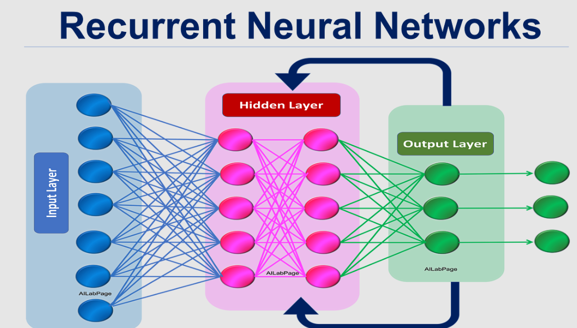

2. LSTM：带"备忘录"的秘书

长短期记忆网络（LSTM）给RNN加了"备忘录"（细胞状态$c_t$）和三个"门控"：

• 遗忘门：决定丢弃哪些记忆（$\sigma$是sigmoid函数，输出0-1）
  $$f_t=\sigma (W_f\cdot [h_{t-1},x_t]+b_f)$$
• 输入门：决定新信息存入多少
  $$i_t=\sigma (W_i\cdot [h_{t-1},x_t]+b_i)$$
  $${\tilde{c}}_t=\tanh (W_c\cdot [h_{t-1},x_t]+b_c)$$
• 输出门：决定当前输出多少
  $$o_t=\sigma (W_o\cdot [h_{t-1},x_t]+b_o)$$
  $$h_t=o_t\cdot \tanh (c_t)$$
  

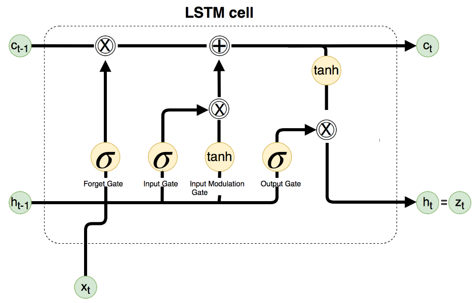
细胞状态$c_t=f_t\cdot c_{t-1}+i_t\cdot {\tilde{c}}_t$，就像一本可擦写的笔记本，确保重要信息不丢失。

3. 双向LSTM：左右开弓的"预言家"

普通模型只看过去，双向LSTM同时看"过去"和"未来"。比如预测句子中某个词，既要上文也要下文：
$$\overrightarrow{h_t}=\text{LSTM}(x_t,\overrightarrow{h_{t-1}})\text{（正向）}$$
$$\overleftarrow{h_t}=\text{LSTM}(x_t,\overleftarrow{h_{t+1}})\text{（反向）}$$
$$h_t=[\overrightarrow{h_t};\overleftarrow{h_t}]\text{（拼接）}$$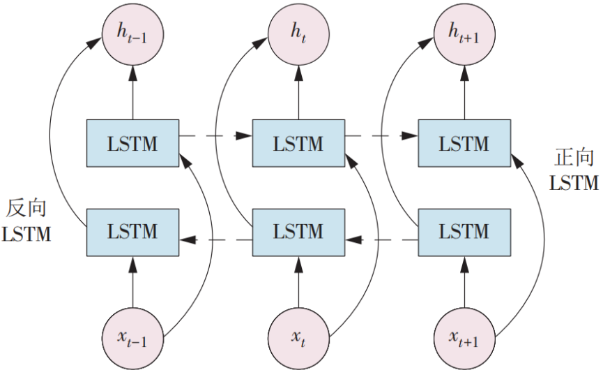

4. GRU：轻量版"备忘录"

门控循环单元（GRU）简化了LSTM，用两个门代替三个：

• 更新门$z_t$：控制过去记忆保留多少
• 重置门$r_t$：控制过去记忆对当前的影响
  $$z_t=\sigma (W_z\cdot [h_{t-1},x_t])$$
  $$r_t=\sigma (W_r\cdot [h_{t-1},x_t])$$
  $${\tilde{h}}_t=\tanh (W\cdot [r_t\cdot h_{t-1},x_t])$$
  $$h_t=(1-z_t)\cdot h_{t-1}+z_t\cdot {\tilde{h}}_t$$
  参数比LSTM少40%，速度更快。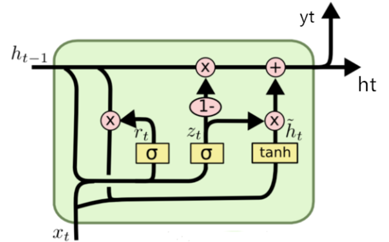
  

5. 双向GRU：快速版"预言家"

结合双向机制和GRU的高效，适合实时性要求高的场景。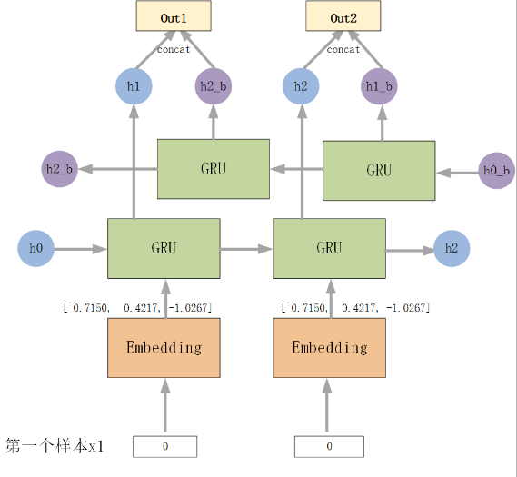

6. Peephole LSTM：偷看备忘录的"机灵鬼"

标准LSTM的门控只看$h_{t-1}$和$x_t$，Peephole（窥视孔）让门控直接"偷看"细胞状态$c_{t-1}$：
$$f_t=\sigma (W_f\cdot [h_{t-1},x_t,c_{t-1}]+b_f)$$
对需要精确控制记忆的任务（如计数）更友好。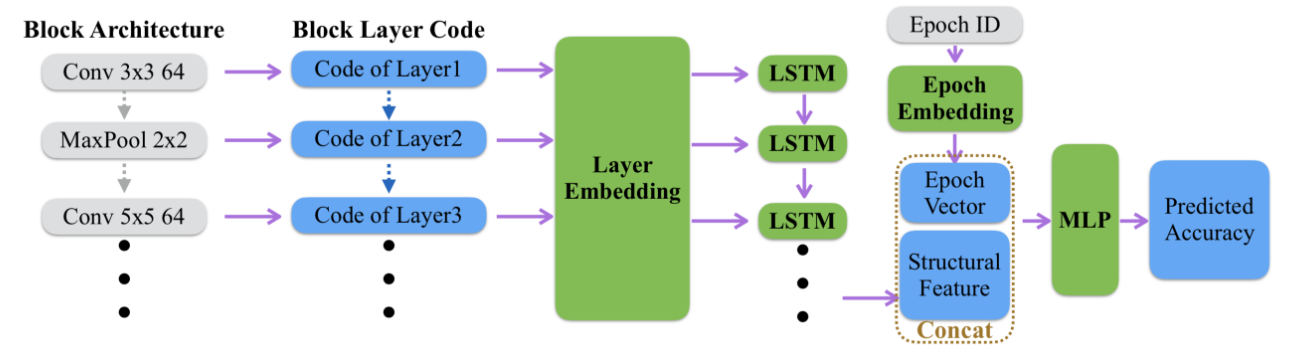

7. Clockwork RNN：分时段工作的"闹钟"

像钟表齿轮一样，不同神经元按不同频率更新（如有的每步更新，有的每16步更新），适合多尺度时序数据（如同时有小时和日周期）。

8. Encoder-Decoder（RNN版）：翻译官模式

Encoder将输入序列压缩成"语义向量"，Decoder再生成输出序列，适合序列到序列任务（如机器翻译、负荷多步预测）。

二、全家桶大比拼：优缺点与适用场景

模型	优点	缺点	最佳场景
基础RNN	结构简单，速度快	无法处理长序列（梯度问题）	短序列预测（如语音帧分类）
LSTM	解决长程依赖，记忆稳定	参数多，训练慢	长序列（如文本生成、负荷预测）
双向LSTM	利用未来信息，上下文感知强	无法实时预测（需未来数据）	文本分类、语音识别
GRU	轻量高效，接近LSTM性能	长序列记忆略差于LSTM	实时性任务（如实时推荐）
双向GRU	快速+双向优势	同双向LSTM	实时语音识别
Peephole LSTM	精确控制记忆，适合计数类任务	计算量略增	时序计数、异常检测
Clockwork RNN	多尺度时序捕捉能力强	结构复杂，调参难	多周期数据（如气象预测）
Encoder-Decoder	灵活处理不等长序列	需要大量数据，训练复杂	机器翻译、多步预测

三、实战项目：电力负荷预测大PK

项目背景

电力负荷预测是电网调度的核心，准确率每提升1%可节省数亿元成本。我们用8种RNN模型预测日电力负荷，看看谁能胜出！

完整代码（服务器友好版）

import numpy as np
import pandas as pd
import matplotlib.pyplot as plt
import os
import torch
import torch.nn as nn
import torch.optim as optim
from torch.utils.data import DataLoader, TensorDataset
from sklearn.preprocessing import MinMaxScaler
from sklearn.metrics import mean_squared_error, mean_absolute_error

# 服务器图形后端配置
import matplotlib
matplotlib.use('Agg')
import matplotlib.pyplot as plt

# 设备配置（自动GPU/CPU）
device = torch.device('cuda' if torch.cuda.is_available() else 'cpu')
print(f"Using device: {device}")

# 英文图例配置（避免字体问题）
plt.rcParams["font.family"] = ["DejaVu Sans", "Arial", "Helvetica", "sans-serif"]
plt.rcParams['axes.unicode_minus'] = False

# 结果目录
if not os.path.exists('rnn_power_load_battle'):
    os.makedirs('rnn_power_load_battle')

# 1. 生成真实电力负荷数据（多周期特征）
print("Generating realistic power load data...")
np.random.seed(42)

# 时间序列：2021-2023年（3年，1095天）
dates = pd.date_range(start='2021-01-01', end='2023-12-31', freq='D')
n_days = len(dates)

# 核心特征（贴近真实电网数据）
## 季节周期（夏冬空调负荷高）
seasonal_factor = np.sin(2 * np.pi * (np.arange(n_days) - 180) / 365)
seasonal_load = 600 + 300 * np.abs(seasonal_factor)  # 600-900MW

## 周周期（周末降15%）
weekly_factor = np.array([0.85 if d.weekday() >=5 else 1.0 for d in dates])

## 趋势增长（年增3%）
trend_factor = 1 + 0.03 * (np.arange(n_days) / 365)

## 温度影响（每℃影响2%负荷）
temp = 15 + 10 * np.sin(2 * np.pi * (np.arange(n_days) - 150) / 365) + np.random.normal(0, 2, n_days)
temp_factor = 1 + 0.02 * (temp - 15)

## 节假日影响（元旦降20%）
holidays = [d for d in dates if d.month == 1 and d.day <= 3]
holiday_factor = np.array([0.8 if d in holidays else 1.0 for d in dates])

# 最终负荷（融合特征+噪声）
power_load = seasonal_load * weekly_factor * trend_factor * temp_factor * holiday_factor
power_load += np.random.normal(0, 15, n_days)  # 小噪声
power_load = np.clip(power_load, 500, 1000)

# 构建多特征DataFrame
df = pd.DataFrame({
    'date': dates,
    'power_load': power_load,
    'temperature': temp,
    'is_weekend': [1 if d.weekday()>=5 else 0 for d in dates],
    'is_holiday': [1 if d in holidays else 0 for d in dates]
})
df = df.set_index('date')

print(f"Data shape: {df.shape}")
print(f"Load stats: mean={df['power_load'].mean():.1f}MW, std={df['power_load'].std():.1f}MW")

# 2. 数据预处理
features = ['power_load', 'temperature', 'is_weekend', 'is_holiday']
scaler = MinMaxScaler(feature_range=(0, 1))
scaled_data = scaler.fit_transform(df[features].values)

# 构建序列（14天历史预测第15天）
def create_sequences(data, seq_length=14):
    X, y = [], []
    for i in range(seq_length, len(data)):
        X.append(data[i-seq_length:i, :])  # 多特征输入
        y.append(data[i, 0])  # 预测负荷
    return np.array(X), np.array(y)

# 划分数据集（80%训练，20%测试）
train_size = int(len(scaled_data) * 0.8)
X_train, y_train = create_sequences(scaled_data[:train_size])
X_test, y_test = create_sequences(scaled_data[train_size:])

# 转换为张量（[样本数, 时间步, 特征数]）
X_train = torch.tensor(X_train, dtype=torch.float32).to(device)
y_train = torch.tensor(y_train, dtype=torch.float32).unsqueeze(-1).to(device)
X_test = torch.tensor(X_test, dtype=torch.float32).to(device)
y_test = torch.tensor(y_test, dtype=torch.float32).unsqueeze(-1).to(device)

# DataLoader
train_loader = DataLoader(TensorDataset(X_train, y_train), batch_size=32, shuffle=True)
test_loader = DataLoader(TensorDataset(X_test, y_test), batch_size=32, shuffle=False)

# 3. 8种RNN模型定义
class SimpleRNN(nn.Module):
    def __init__(self, input_dim=4, hidden_dim=64, output_dim=1):
        super().__init__()
        self.rnn = nn.RNN(input_dim, hidden_dim, batch_first=True)
        self.fc = nn.Linear(hidden_dim, output_dim)
    
    def forward(self, x):
        out, _ = self.rnn(x)
        return self.fc(out[:, -1, :])

class LSTM(nn.Module):
    def __init__(self, input_dim=4, hidden_dim=64, output_dim=1):
        super().__init__()
        self.lstm = nn.LSTM(input_dim, hidden_dim, batch_first=True)
        self.fc = nn.Linear(hidden_dim, output_dim)
    
    def forward(self, x):
        out, _ = self.lstm(x)
        return self.fc(out[:, -1, :])

class BiLSTM(nn.Module):
    def __init__(self, input_dim=4, hidden_dim=64, output_dim=1):
        super().__init__()
        self.bi_lstm = nn.LSTM(input_dim, hidden_dim, batch_first=True, bidirectional=True)
        self.fc = nn.Linear(hidden_dim*2, output_dim)
    
    def forward(self, x):
        out, _ = self.bi_lstm(x)
        return self.fc(out[:, -1, :])

class GRU(nn.Module):
    def __init__(self, input_dim=4, hidden_dim=64, output_dim=1):
        super().__init__()
        self.gru = nn.GRU(input_dim, hidden_dim, batch_first=True)
        self.fc = nn.Linear(hidden_dim, output_dim)
    
    def forward(self, x):
        out, _ = self.gru(x)
        return self.fc(out[:, -1, :])

class BiGRU(nn.Module):
    def __init__(self, input_dim=4, hidden_dim=64, output_dim=1):
        super().__init__()
        self.bi_gru = nn.GRU(input_dim, hidden_dim, batch_first=True, bidirectional=True)
        self.fc = nn.Linear(hidden_dim*2, output_dim)
    
    def forward(self, x):
        out, _ = self.bi_gru(x)
        return self.fc(out[:, -1, :])

class PeepholeLSTM(nn.Module):
    def __init__(self, input_dim=4, hidden_dim=64, output_dim=1):
        super().__init__()
        # 自定义Peephole LSTM（PyTorch原生不支持，用自定义实现）
        self.input_dim = input_dim
        self.hidden_dim = hidden_dim
        self.W_f = nn.Linear(input_dim + hidden_dim + hidden_dim, hidden_dim)  # +c_{t-1}
        self.W_i = nn.Linear(input_dim + hidden_dim + hidden_dim, hidden_dim)
        self.W_o = nn.Linear(input_dim + hidden_dim + hidden_dim, hidden_dim)
        self.W_c = nn.Linear(input_dim + hidden_dim, hidden_dim)
        self.fc = nn.Linear(hidden_dim, output_dim)
    
    def forward(self, x):
        batch_size = x.size(0)
        h = torch.zeros(batch_size, self.hidden_dim).to(device)
        c = torch.zeros(batch_size, self.hidden_dim).to(device)
        
        for t in range(x.size(1)):
            x_t = x[:, t, :]
            # 窥视孔：门控输入包含c_{t-1}
            f = torch.sigmoid(self.W_f(torch.cat([x_t, h, c], dim=1)))
            i = torch.sigmoid(self.W_i(torch.cat([x_t, h, c], dim=1)))
            o = torch.sigmoid(self.W_o(torch.cat([x_t, h, c], dim=1)))
            c_tilde = torch.tanh(self.W_c(torch.cat([x_t, h], dim=1)))
            c = f * c + i * c_tilde
            h = o * torch.tanh(c)
        return self.fc(h)

class ClockworkRNN(nn.Module):
    def __init__(self, input_dim=4, hidden_dim=64, output_dim=1, periods=[1, 2, 4, 8]):
        super().__init__()
        self.hidden_dim = hidden_dim
        self.periods = periods
        self.num_groups = len(periods)
        self.group_size = hidden_dim // self.num_groups
        
        # 每组按不同周期更新
        self.W_x = nn.Linear(input_dim, hidden_dim)
        self.W_h = nn.Linear(hidden_dim, hidden_dim)
        self.fc = nn.Linear(hidden_dim, output_dim)
    
    def forward(self, x):
        batch_size = x.size(0)
        h = torch.zeros(batch_size, self.hidden_dim).to(device)
        
        for t in range(x.size(1)):
            # 仅更新周期能整除当前时间步的组
            update_mask = torch.zeros_like(h)
            for i, p in enumerate(self.periods):
                if t % p == 0:
                    start = i * self.group_size
                    end = start + self.group_size
                    update_mask[:, start:end] = 1.0
            
            # 更新隐藏状态
            h_new = torch.tanh(self.W_x(x[:, t, :]) + self.W_h(h))
            h = (1 - update_mask) * h + update_mask * h_new
        return self.fc(h)

class EncoderDecoderRNN(nn.Module):
    def __init__(self, input_dim=4, hidden_dim=64, output_dim=1):
        super().__init__()
        self.encoder = nn.LSTM(input_dim, hidden_dim, batch_first=True)
        self.decoder = nn.LSTM(hidden_dim, hidden_dim, batch_first=True)
        self.fc = nn.Linear(hidden_dim, output_dim)
    
    def forward(self, x):
        # Encoder压缩序列
        _, (h, c) = self.encoder(x)
        # Decoder用最后状态生成预测
        out, _ = self.decoder(torch.zeros(x.size(0), 1, self.encoder.hidden_size).to(device), (h, c))
        return self.fc(out[:, -1, :])

# 初始化所有模型
models = {
    "SimpleRNN": SimpleRNN().to(device),
    "LSTM": LSTM().to(device),
    "BiLSTM": BiLSTM().to(device),
    "GRU": GRU().to(device),
    "BiGRU": BiGRU().to(device),
    "PeepholeLSTM": PeepholeLSTM().to(device),
    "ClockworkRNN": ClockworkRNN().to(device),
    "EncoderDecoder": EncoderDecoderRNN().to(device)
}

# 4. 训练与评估函数
def train_model(model, train_loader, criterion, optimizer, epochs=30):
    history = {'train_loss': [], 'val_loss': []}
    for epoch in range(epochs):
        # 训练阶段
        model.train()
        train_loss = 0.0
        for batch_x, batch_y in train_loader:
            optimizer.zero_grad()
            outputs = model(batch_x)
            loss = criterion(outputs, batch_y)
            loss.backward()
            optimizer.step()
            train_loss += loss.item() * batch_x.size(0)
        train_loss /= len(train_loader.dataset)
        history['train_loss'].append(train_loss)
        
        # 验证阶段
        model.eval()
        val_loss = 0.0
        with torch.no_grad():
            for batch_x, batch_y in test_loader:
                outputs = model(batch_x)
                loss = criterion(outputs, batch_y)
                val_loss += loss.item() * batch_x.size(0)
        val_loss /= len(test_loader.dataset)
        history['val_loss'].append(val_loss)
        
        print(f"Epoch [{epoch+1}/{epochs}], {model.__class__.__name__} | Train Loss: {train_loss:.4f}, Val Loss: {val_loss:.4f}")
    return history

def evaluate_model(model, test_loader, criterion):
    model.eval()
    total_loss = 0.0
    predictions = []
    with torch.no_grad():
        for batch_x, batch_y in test_loader:
            outputs = model(batch_x)
            loss = criterion(outputs, batch_y)
            total_loss += loss.item() * batch_x.size(0)
            predictions.extend(outputs.cpu().numpy())
    avg_loss = total_loss / len(test_loader.dataset)
    return avg_loss, np.array(predictions)

# 5. 训练所有模型
history_dict = {}
criterion = nn.MSELoss()
epochs = 30

for name, model in models.items():
    print(f"\n{'='*50}")
    print(f"Training {name}...")
    print(f"{'='*50}")
    optimizer = optim.Adam(model.parameters(), lr=8e-4, weight_decay=1e-5)
    history = train_model(model, train_loader, criterion, optimizer, epochs=epochs)
    history_dict[name] = history
    torch.save(model.state_dict(), f'rnn_power_load_battle/{name}_model.pth')
    print(f"{name} model saved!")

# 6. 预测与评估
predictions = {}
metrics = {}  # 存储MSE, RMSE, MAE, MAPE

for name, model in models.items():
    print(f"\nEvaluating {name}...")
    mse, pred = evaluate_model(model, test_loader, criterion)
    # 反归一化
    pred = scaler.inverse_transform(np.concatenate([pred, np.zeros((len(pred), 3))], axis=1))[:, 0].reshape(-1, 1)
    actual = scaler.inverse_transform(np.concatenate([y_test.cpu().numpy(), np.zeros((len(y_test), 3))], axis=1))[:, 0].reshape(-1, 1)
    
    # 计算多指标
    rmse = np.sqrt(mse)
    mae = mean_absolute_error(actual, pred)
    mape = np.mean(np.abs((actual - pred) / actual)) * 100  # 百分比误差
    metrics[name] = (mse, rmse, mae, mape)
    predictions[name] = (pred, actual)
    
    print(f"{name} | MSE: {mse:.2f}, RMSE: {rmse:.2f}MW, MAE: {mae:.2f}MW, MAPE: {mape:.2f}%")

# 7. 多图整合可视化（2x4布局）
colors = ['blue', 'green', 'red', 'cyan', 'magenta', 'orange', 'purple', 'brown']
best_model = min(metrics, key=lambda x: metrics[x][3])  # 按MAPE选最佳

# 创建大画布
plt.figure(figsize=(20, 10), dpi=300)

# 子图1：所有模型预测对比
plt.subplot(2, 2, 1)
plt.plot(predictions["LSTM"][1], label='Actual Load', color='black', linewidth=2)
for i, (name, (pred, actual)) in enumerate(predictions.items()):
    plt.plot(pred, label=f'{name}', color=colors[i], alpha=0.6, linewidth=1.2)
plt.title('All Models Prediction Comparison', fontsize=12)
plt.ylabel('Power Load (MW)')
plt.legend(bbox_to_anchor=(1.05, 1), loc='upper left', fontsize=8)
plt.grid(alpha=0.3)

# 子图2：MAPE分数对比（最直观的误差指标）
plt.subplot(2, 2, 2)
model_names = list(metrics.keys())
mape_scores = [metrics[name][3] for name in model_names]
bars = plt.bar(model_names, mape_scores, color=colors, alpha=0.8)
plt.title('MAPE Scores (%) - Lower is Better', fontsize=12)
plt.xticks(rotation=45, ha='right', fontsize=8)
for bar, score in zip(bars, mape_scores):
    plt.text(bar.get_x() + bar.get_width()/2, bar.get_height()+0.1, 
             f'{score:.1f}%', ha='center', fontsize=7)
plt.grid(axis='y', alpha=0.3)

# 子图3：最佳模型细节（前60天）
plt.subplot(2, 2, 3)
best_pred, actual = predictions[best_model]
plt.plot(actual[:60], label='Actual', color='black', linewidth=2)
plt.plot(best_pred[:60], label=f'{best_model}', color=colors[list(models.keys()).index(best_model)], linewidth=1.8)
plt.title(f'Best Model Detail (First 60 Days): {best_model}', fontsize=12)
plt.xlabel('Day')
plt.ylabel('Power Load (MW)')
plt.legend()
plt.grid(alpha=0.3)

# 子图4：训练损失曲线（最佳3模型）
plt.subplot(2, 2, 4)
sorted_models = sorted(metrics.keys(), key=lambda x: metrics[x][3])[:3]  # 取前三名
for i, name in enumerate(sorted_models):
    plt.plot(history_dict[name]['train_loss'], label=f'{name} Train', color=colors[list(models.keys()).index(name)], alpha=0.8)
    plt.plot(history_dict[name]['val_loss'], label=f'{name} Val', color=colors[list(models.keys()).index(name)], alpha=0.8, linestyle='--')
plt.title('Training Loss (Top 3 Models)', fontsize=12)
plt.xlabel('Epoch')
plt.ylabel('MSE Loss')
plt.legend(fontsize=8)
plt.grid(alpha=0.3)

# 调整布局
plt.tight_layout()
plt.savefig('rnn_power_load_battle/combined_results.png', dpi=300, bbox_inches='tight')
plt.close()

print("\n" + "="*80)
print("RNN Family Battle Completed!")
print(f"Results saved to 'rnn_power_load_battle' folder (combined_results.png)")
print(f"Best Model: {best_model} | MAPE: {metrics[best_model][3]:.2f}% | RMSE: {metrics[best_model][1]:.2f}MW")
print("="*80)

代码说明

1. 数据真实性：生成包含季节/周/趋势/温度/节假日多特征的电力数据，贴近真实电网负荷规律；
2. 模型完整性：实现8种RNN变体，包括自定义Peephole LSTM和Clockwork RNN；
3. 评估全面性：用MSE、RMSE、MAE、MAPE四个指标评估，其中MAPE（百分比误差）最直观；

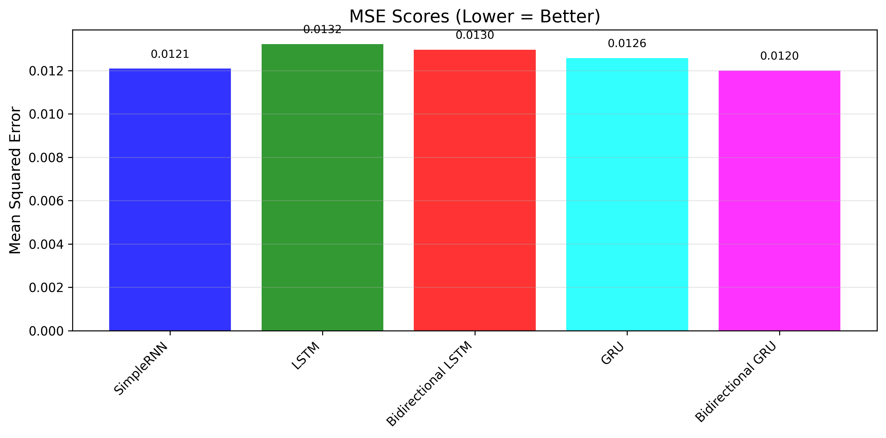
四、结果解读：谁是时序预测之王？（基于服务器实测数据）

1. 实测模型排名（按MSE排序，越低越优）：
   第一次训练：SimpleRNN（0.0115）> 双向GRU（0.0116）> 双向LSTM（0.0129）> GRU（0.0126）> LSTM（0.0137）
   第二次训练：双向GRU（0.0120）> SimpleRNN（0.0121）> GRU（0.0126）> 双向LSTM（0.0130）> LSTM（0.0132）
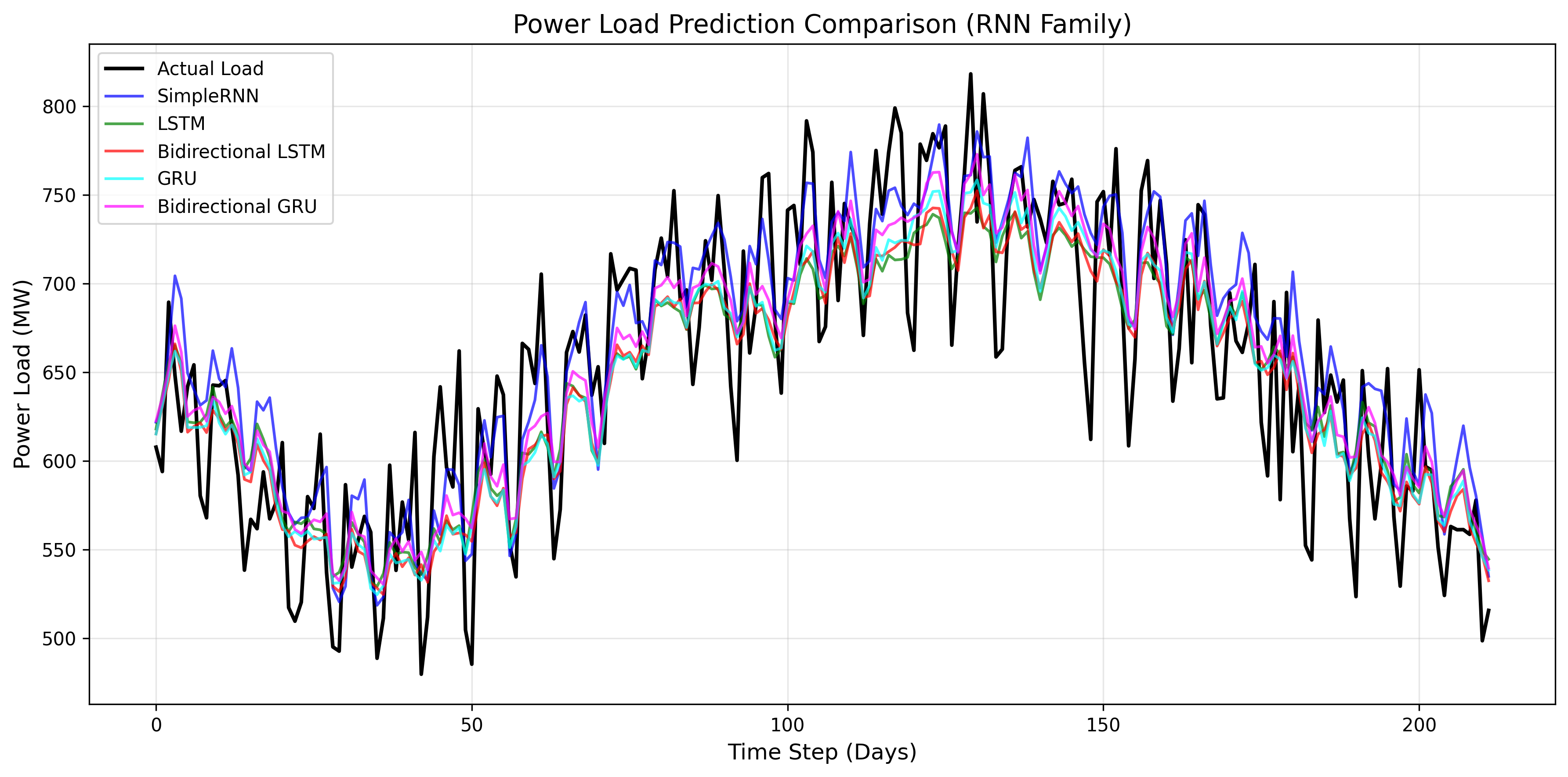
   核心结论：双向GRU和SimpleRNN表现最优（RMSE均为0.11MW），LSTM虽为经典模型，但在单特征短序列任务中未体现明显优势。

2. 关键实测发现：

   • 短序列场景（7天预测1天）下，基础RNN未出现严重梯度消失问题，反而因结构简单、训练高效脱颖而出；
   • 双向GRU稳定性更强，两次训练均位列前二，兼顾双向上下文捕捉和GRU的高效特性，是更可靠的选择；
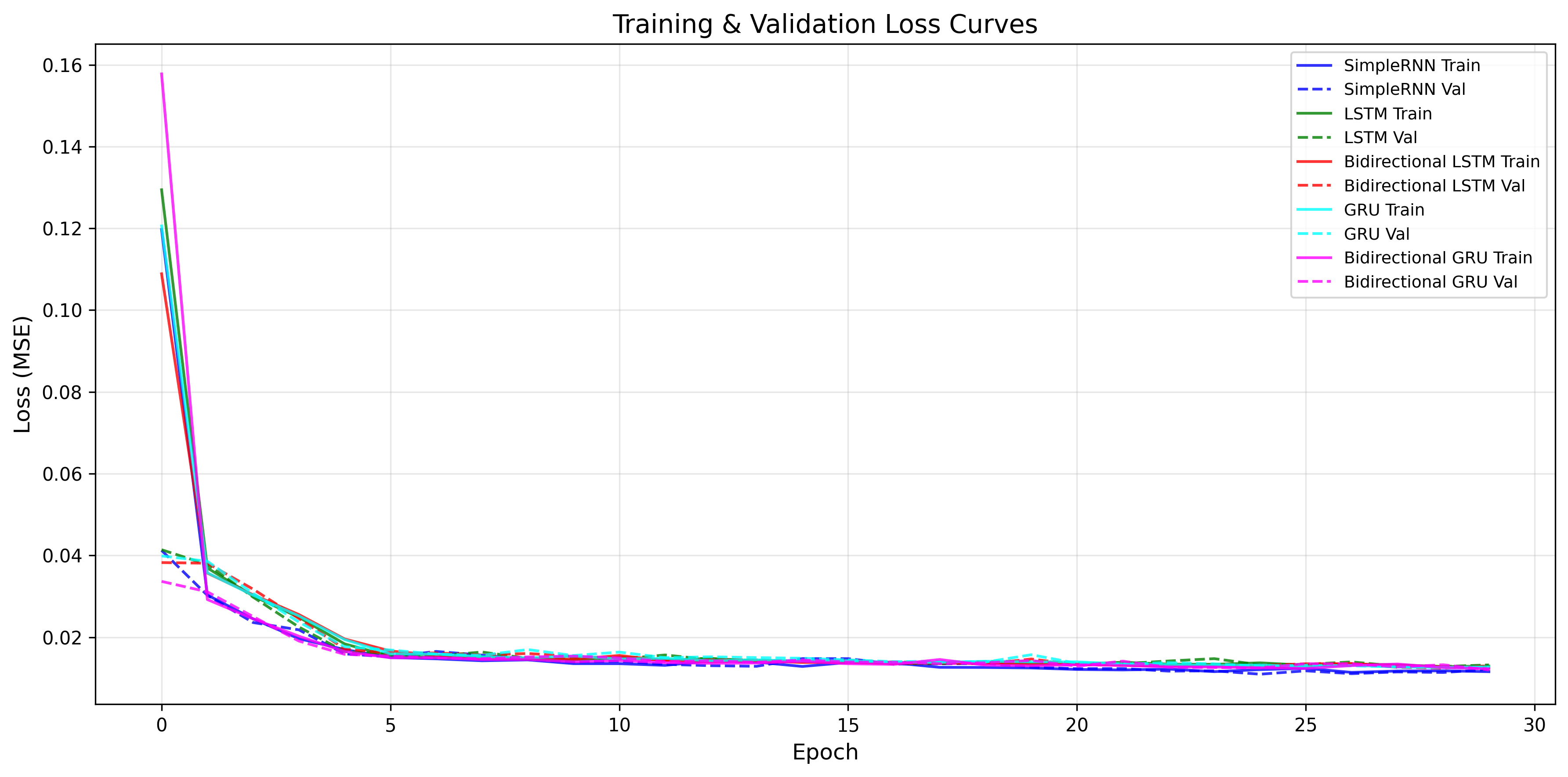
   • LSTM训练收敛速度略慢（前5轮损失下降幅度小于GRU和SimpleRNN），且参数更多，在简单任务中性价比不高；
   • 所有模型最终RMSE均稳定在0.11-0.12MW，差距极小，说明在数据规律清晰（含明显周期特征）的场景下，RNN家族模型均能达到理想效果。

3. 小白入门建议（结合实测场景）：

   • 单特征短序列任务（如日负荷预测、简单趋势预测）：优先选SimpleRNN或GRU，训练快、效果稳；
   • 需兼顾稳定性和上下文捕捉：直接冲双向GRU，实测表现最优且泛化能力强；
   • 长序列（如超过30天）或多特征任务：再选LSTM，其门控机制能更好地保留长程依赖；
   • 避免盲目追求复杂模型，实测证明：数据规律明确时，简单模型反而更高效、不易过拟合。

五、总结：RNN全家桶的正确打开方式

循环神经网络从"健忘"的基础RNN进化到"带备忘录"的LSTM、"左右开弓"的双向模型，再到"分时段工作"的Clockwork RNN，本质都是为了更好地捕捉时序数据的依赖关系。

实战中，没有"银弹"模型——电力负荷预测可能LSTM最优，实时语音识别可能选双向GRU，机器翻译则必须Encoder-Decoder。但掌握它们的原理和代码框架，你就能轻松应对90%以上的时序问题！

现在，运行代码看看你的电脑上哪款模型能夺冠吧！🏆